MAST
Tie Constraints

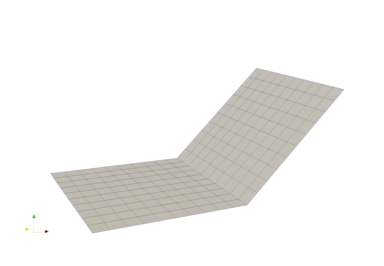
This example solves a cantilever rectangular plate with a uniformly distributed load on the top of the plate.

An inclined section is created as a separate mesh and connected to the plate using tie constraints at the shared edge.

For direct solver, run with options: -ksp_type preonly -pc_type lu

Mesh Generation

 This function initializes the mesh data stucture. 
void init_mesh(libMesh::ReplicatedMesh& mesh) {

A square $ 0.3m \times 0.3m $ mesh is created with QUAD4 elements.

length = 0.3,
width = 0.3,
pi = acos(-1.);

The mesh generation tools from libMesh are used to initialize this section of the mesh. A $ 10\times 10 $ mesh of QUAD4 elements is used for discretization.

libMesh::MeshTools::Generation::build_square(mesh, 10, 10, 0.0, length, 0.0, width, libMesh::QUAD4);

Next, a section of the same dimension and mesh density is created and added to the mesh object. This section is attached to the right side of the cantilever section (created above) using kinematic constraints. The section is inclined at a $ 45^\circ $ angle.

example_4_mesh.png
std::map<const libMesh::Node*, libMesh::Node*>
node_map;

add new nodes

libMesh::MeshBase::const_node_iterator
n_it = mesh.nodes_begin(),
n_end = mesh.nodes_end();
for ( ; n_it != n_end; n_it++) {
const libMesh::Node* nd = *n_it;
libMesh::Node* new_nd = libMesh::Node::build(*nd, libMesh::DofObject::invalid_id).release();

add new node to the map so that we will be able to use it during element creation below

node_map[nd] = new_nd;

modify the coordinates to include the incline.

(*new_nd)(0) = length + (*nd)(0)*cos(pi/4.);
(*new_nd)(1) += 0.;
(*new_nd)(2) = (*nd)(0)*sin(pi/4.);
}

add new nodes

std::map<const libMesh::Node*, libMesh::Node*>::iterator
nd_map_it = node_map.begin(),
nd_map_end = node_map.end();
for ( ; nd_map_it != nd_map_end; nd_map_it++)
mesh.add_node(nd_map_it->second);

add new elements

std::set<libMesh::Elem*> elems;
libMesh::MeshBase::const_element_iterator
e_it = mesh.elements_begin(),
e_end = mesh.elements_end();
for ( ; e_it != e_end; e_it++) {
const libMesh::Elem* e = *e_it;
libMesh::Elem* new_e = libMesh::Elem::build(e->type()).release();

set nodes

for (unsigned int i=0; i<e->n_nodes(); i++)
new_e->set_node(i) = node_map[e->node_ptr(i)];

set subdomain ID to 1

new_e->subdomain_id() = e->subdomain_id()+1;

set boundary IDs

for (unsigned short int n=0; n<e->n_sides(); n++) {
if (mesh.boundary_info->n_boundary_ids(e, n)) {

add the boundary tags to the panel mesh

std::vector<libMesh::boundary_id_type> bc_ids;
mesh.boundary_info->boundary_ids(e, n, bc_ids);
for ( unsigned int bid=0; bid < bc_ids.size(); bid++)
mesh.boundary_info->add_side(new_e, n, bc_ids[bid]+4);
}
}
elems.insert(new_e);
}
std::set<libMesh::Elem*>::iterator
elem_set_it = elems.begin(),
elem_set_end = elems.end();
for ( ; elem_set_it != elem_set_end; elem_set_it++)
mesh.add_elem(*elem_set_it);
mesh.prepare_for_use();

the boundaries are indentified using the following tags.

mesh.boundary_info->sideset_name(4) = "bottom2";
mesh.boundary_info->sideset_name(5) = "right2";
mesh.boundary_info->sideset_name(6) = "top2";
mesh.boundary_info->sideset_name(7) = "left2";
}
int main(int argc, const char** argv)
{

Initialize libMesh library.

libMesh::LibMeshInit init(argc, argv);

A replicated mesh is used, which will store the entire mesh on all elements.

libMesh::ReplicatedMesh mesh(init.comm());

Initialize the mesh using the function defined above.

init_mesh(mesh);
mesh.print_info();

System Initialization

Create EquationSystems object, which is a container for multiple systems of equations that are defined on a given mesh.

libMesh::EquationSystems equation_systems(mesh);

Add system of type MAST::NonlinearSystem (which wraps libMesh::NonlinearImplicitSystem) to the EquationSystems container. We name the system "structural" and also get a reference to the system so we can easily reference it later.

MAST::NonlinearSystem & system = equation_systems.add_system<MAST::NonlinearSystem>("structural");

Create a finite element type for the system. Here we use first order Lagrangian-type finite elements.

libMesh::FEType fetype(libMesh::FIRST, libMesh::LAGRANGE);

Initialize the system to the correct set of variables for a structural analysis. In libMesh this is analogous to adding variables (each with specific finite element type/order to the system for a particular system of equations.

MAST::StructuralSystemInitialization structural_system(system,
system.name(),
fetype);

Initialize a new structural discipline using equation_systems.

MAST::PhysicsDisciplineBase discipline(equation_systems);

Dirichlet Boundary Condition

Create and add boundary conditions to the structural system. A Dirichlet BC adds fixed displacement BCs. Here we use the side boundary ID numbering created by the libMesh generator to clamp the edge of the mesh along x=0.0. We apply the BC to all variables on each node in the subdomain ID 0, which clamps this edge.

MAST::DirichletBoundaryCondition clamped_edge0, clamped_edge1, clamped_edge2, clamped_edge3; // Create BC object.
std::vector<unsigned int> vars = {0, 1, 2, 3, 4, 5};
clamped_edge3.init(3, vars); // Assign boundary ID and variables to constrain
discipline.add_dirichlet_bc(3, clamped_edge3); // Attach boundary condition to discipline
discipline.init_system_dirichlet_bc(system); // Initialize the BC in the system.

Initialize the equation system since we now know the size of our system matrices (based on mesh, element type, variables in the structural_system) as well as the setup of dirichlet boundary conditions. This initialization process is basically a pre-processing step to preallocate storage and spread it across processors.

Kinematic Coupling

The tie constraints are added through the DofConstraintRow functionality in libMesh. Here, constraint equations are specified between degrees-of-freedom (DoFs). The first step in the coupling is identified through a geometric search which identifies the nodes on the respective boundaries of master and slave mesh that need to be coupled with each other. Here, the right boundary (boundary id 1) of the cantilevered plate is connected to the left boundary (boundary id 7) of the unconnected domain. Once the nodes have been identified, the next step is to identify the constraint equations that will define the dependence of the slave nodes on the master nodes. This is done by the MeshCouplingBase class. The constraint equations are then provided to libMesh through this ad-hoc class Constr below.

class Constr: public libMesh::System::Constraint {
public:
Constr(MAST::KinematicCoupling& kin_coupling): _kin_coupling(kin_coupling) {}
virtual ~Constr () {}
virtual void constrain () { _kin_coupling.add_dof_constraints_to_dof_map(); }
protected:
MAST::KinematicCoupling& _kin_coupling;
};

The MeshCouplingBase class will used to couple the boudnary ID 7 as the slave to the boundary ID 1 as the master. A geometric search will be used to identify node couplings within a circular radius of 0.005 m.

MAST::MeshCouplingBase mesh_coupling(structural_system);

This call will lead to a master-slave boundary-to-boundary coupling. This can be uncommented and the next boundary-to-subdomain call can be commented to enable this call. mesh_coupling.add_master_and_slave_boundary_coupling(1, 7, .005);

the mesh can also be coupled using slave-boundary to master-subdomain coupling.

mesh_coupling.add_slave_boundary_and_master_subdomain_coupling(0, 7, .005);

The KinematicCoupling class uses the search results to create the kinematic constraints (or tie-constraints) for libMesh::DofMap

MAST::KinematicCoupling kin_coupling(structural_system);
kin_coupling.add_master_and_slave(mesh_coupling.get_node_couplings(), true);

This class will is provided to libMesh::System and it will be called by libMesh when the system is initialized.

Constr kc(kin_coupling);
system.attach_constraint_object(kc);

This will initialize the DoFs, Dirichlet Constraints and kinematic constraints.

equation_systems.init();
equation_systems.print_info();

Load and Property Definition

Create parameters.

MAST::Parameter thickness("th", 0.001);
MAST::Parameter E("E", 72.e9);
MAST::Parameter nu("nu", 0.33);
MAST::Parameter rho("rho", 2700.);
MAST::Parameter kappa("kappa", 5./6.);
MAST::Parameter alpha("alpha", 1.5e-5);
MAST::Parameter zero("zero", 0.0);
MAST::Parameter pressure1("p", 1.0e2);
MAST::Parameter pressure2("p", -1.0e2);
MAST::Parameter temperature("T", 0.0);

Create ConstantFieldFunctions used to spread parameters throughout the model.

MAST::ConstantFieldFunction th_f("h", thickness);
MAST::ConstantFieldFunction rho_f("rho", rho);
MAST::ConstantFieldFunction kappa_f("kappa", kappa);
MAST::ConstantFieldFunction alpha_f("alpha_expansion", alpha);
MAST::ConstantFieldFunction off_f("off", zero);
MAST::ConstantFieldFunction pressure1_f("pressure", pressure1);
MAST::ConstantFieldFunction pressure2_f("pressure", pressure2);
MAST::ConstantFieldFunction temperature_f("temperature", temperature);
MAST::ConstantFieldFunction ref_temp_f("ref_temperature", zero);

Initialize load. The same pressure is applied to both sub-domains 1 and 2.

surface_pressure1.add(pressure1_f);
surface_pressure2.add(pressure2_f);
discipline.add_volume_load(0, surface_pressure1);
discipline.add_volume_load(1, surface_pressure2);
temperature_load.add(temperature_f);
temperature_load.add(ref_temp_f);
discipline.add_volume_load(0, temperature_load);
discipline.add_volume_load(1, temperature_load);

Create the material property card ("card" is NASTRAN lingo) and the relevant parameters to it. An isotropic material needs elastic modulus (E) and Poisson ratio (nu) to describe its behavior.

material.add(E_f);
material.add(nu_f);
material.add(kappa_f);
material.add(alpha_f);
material.add(rho_f);

Create the section property card. Attach all property values.

section.add(th_f);
section.add(off_f);

Attach material to the card.

section.set_material(material);

Initialize the specify the subdomain in the mesh that it applies to.

discipline.set_property_for_subdomain(0, section);
discipline.set_property_for_subdomain(1, section);

Solution

Create nonlinear assembly object and set the discipline and structural_system. Create reference to system.

assembly.set_discipline_and_system(discipline, structural_system);
elem_ops.set_discipline_and_system(discipline, structural_system);
MAST::NonlinearSystem& nonlinear_system = assembly.system();

Zero the solution before solving.

nonlinear_system.solution->zero();
nonlinear_system.solve(elem_ops, assembly);

post-process the stress for plotting. This is done through the output and stress assembly classes.

MAST::StressAssembly stress_assembly;
stress.set_discipline_and_system (discipline, structural_system);
stress_assembly.set_discipline_and_system(discipline, structural_system);
stress_assembly.update_stress_strain_data(stress, *system.solution);

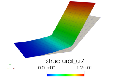
Following is a the displacement contour of the panel with the undeformed mesh plotted for reference. The displacement continuity at the interface is properly enforced.

example_4_uz_contour.png
libMesh::ExodusII_IO(mesh).write_equation_systems("panel.exo", equation_systems);